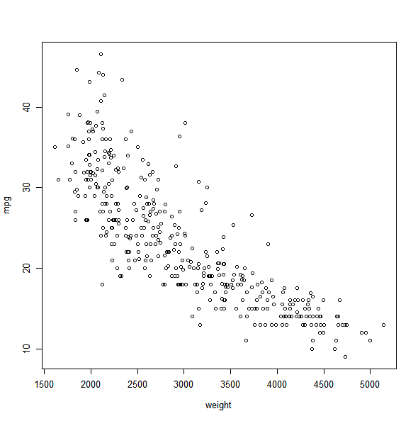
We can use the plot() function to produce scatterplots of the quantitative
variables.
plot(weight, mpg)
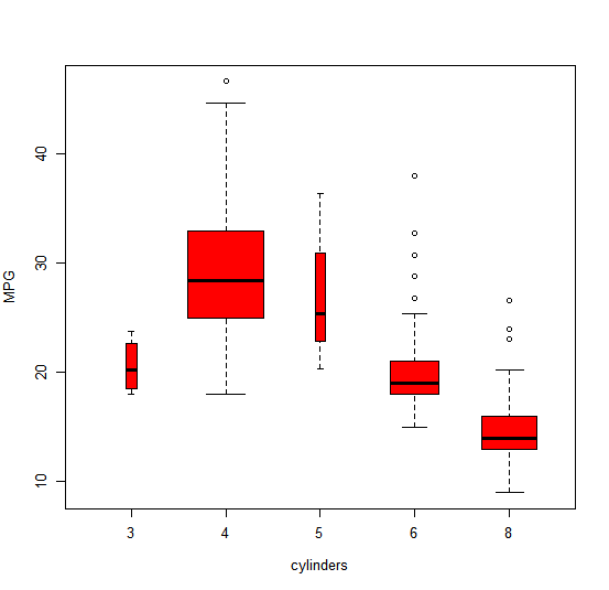
If the variable plotted on the x-axis is categorical, then boxplots will
automatically be produced by the plot() function (remember that in Loading data 4 we turned cylinders in a qualitative variable).
As usual, a number of options can be specified in order to customize the plots (col for customizing the color, varwidth to have variable width of the boxplots depending on the amount of observations in each category, and xlab and ylab for axis descriptions).
plot(cylinders, mpg, col = "red", varwidth = T, xlab = "cylinders", ylab = "MPG")
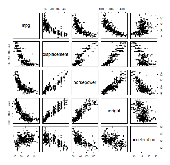
The pairs() function creates a scatterplot matrix i.e. a scatterplot for every
pair of variables for any given data set.
pairs(Auto)
We can also produce a scatterplot matrix for just a subset of the variables.
pairs(~mpg +
  displacement +
  horsepower +
  weight +
  acceleration, Auto)
hist(mpg, col = 2, breaks = 15)
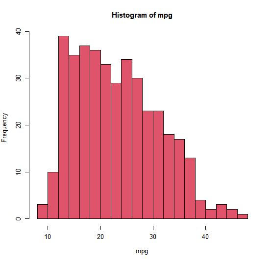
The hist() function can be used to plot a histogram. Note that col = 2
histogram has the same effect as col = "red". breaks = 15 gives us 15 separate bins.
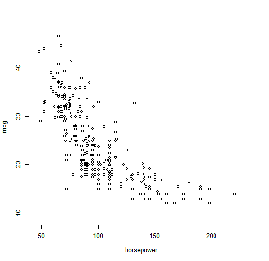
In conjunction with the plot() function, identify() provides a useful
interactive method for identifying the value for a particular variable for
points on a plot. We pass in three arguments to identify(): the x-axis
variable, the y-axis variable, and the variable whose values we would like
to see printed for each point. Then clicking on a given point in the plot
will cause R to print the value of the variable of interest. Right-clicking on
the plot will exit the identify() function (control-click on a Mac). The
numbers printed under the identify() function correspond to the rows for
the selected points.
plot(horsepower, mpg)
identify(horsepower, mpg, name)
The summary() function produces a numerical summary of each variable in
a particular data set.
> summary(Auto)
      mpg         cylinders      displacement
Min.    : 9.00  Min .   :3.000  Min.    : 68.0
1st Qu .:17.00  1st Qu .:4.000  1st Qu .:105.0
Median  :22.75  Median  :4.000  Median  :151.0
Mean    :23.45  Mean    :5.472   Mean   :194.4
3rd Qu .:29.00  3rd Qu .:8.000  3rd Qu .:275.8
Max.    :46.60  Max .   :8.000  Max.    :455.0

   horsepower       weight       acceleration
Min.    : 46.0  Min .   :1613   Min .   : 8.00
1st Qu. : 75.0  1st Qu .:2225   1st Qu .:13.78
Median  : 93.5  Median  :2804   Median  :15.50
Mean    :104.5  Mean    :2978   Mean    :15.54
3rd Qu .:126.0  3rd Qu .:3615   3rd Qu .:17.02
Max.    :230.0  Max .   :5140   Max .   :24.80

    year            origin              name
Min.    :70.00  Min .   :1.000  amc matador         : 5
1st Qu .:73.00  1st Qu .:1.000  ford pinto          : 5
Median  :76.00  Median  :1.000  toyota corolla      : 5
Mean    :75.98  Mean    :1.577  amc gremlin         : 4
3rd Qu .:79.00  3rd Qu .:2.000  amc hornet          : 4
Max.    :82.00  Max .   :3.000  chevrolet chevette  : 4
                                (Other) :365
For qualitative variables such as name, R will list the number of observations
that fall in each category. We can also produce a summary of just a single
variable.
Once we have finished using R, we type q() in order to shut it down, or
quit. When exiting R, we have the option to save the current workspace so
that all objects (such as data sets) that we have created in this R session
will be available next time. Before exiting R, we may want to save a record
of all of the commands that we typed in the most recent session; this can
be accomplished using the savehistory() function. Next time we enter R,
we can load that history using the loadhistory() function.
Questions
Answer the following multiple choice questions by assigning the value 1, 2, 3 or 4 to the question title.
For example:
- MC1:
A) Bananas are yellow.
B) Tomatoes are blue.- 1) Both statements are true.
- 2) Both statements are false.
- 3) A is true and B is false.
- 4) A is false and B is true.
- MC2:
A) Oranges are purple.
B) Apples are pink.- 1) Both statements are true.
- 2) Both statements are false.
- 3) A is true and B is false.
- 4) A is false and B is true.
MC1 = 3
MC2 = 2
- MC1:
A) The scatterplot where weight is plotted against mpg suggests that there is a quadratic relationship between weight and mpg
B) The boxplots where cylinders are plotted against mpg suggests that vehicles with eight cylinders are most fuel efficient- 1) Both statements are true.
- 2) Both statements are false.
- 3) A is true and B is false.
- 4) A is false and B is true.