We implement partial least squares (PLS) using the plsr() function, also
in the pls library. The syntax is just like that of the pcr() function.
> set.seed(1)
> pls.fit <- plsr(Salary ~ ., data = Hitters, subset = train, scale = TRUE, validation = "CV")
> summary(pls.fit)
Data: 	X dimension: 131 19
	Y dimension: 131 1
Fit method: kernelpls
Number of components considered: 19

VALIDATION: RMSEP
Cross-validated using 10 random segments.
       (Intercept)  1 comps  2 comps  3 comps  4 comps
CV           428.3    325.5    329.9    328.8    339.0
adjCV        428.3    325.0    328.2    327.2    336.6
...

TRAINING: % variance explained
        1 comps  2 comps  3 comps  4 comps  5 comps
X         39.13    48.80    60.09    75.07    78.58
Salary    46.36    50.72    52.23    53.03    54.07
...
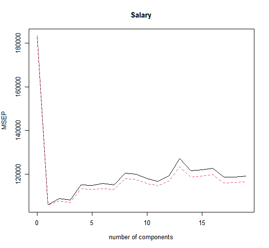
One can also plot the cross-validation scores using the validationplot() function. Using val.type="MSEP" will cause the cross-validation MSE to be plotted:
> validationplot(pls.fit, val.type = "MSEP")

The lowest cross-validation error occurs when only \(M = 1\) partial least squares directions are used. We now evaluate the corresponding test set \(MSE\).
> pls.pred <- predict(pls.fit, x[test,], ncomp = 1)
> mean((pls.pred - y.test)^2)
[1] 151995
The test \(MSE\) is comparable to, but slightly higher than, the test \(MSE\) obtained using ridge regression, the lasso, and PCR.
Questions
- Using the
Bostondataset, try creating a PLS model with cross validation and store it inpls.fit. - Use the summary of the fitted model in order to determine the value of \(M\) where \(MSE\) is minimized.
- With that value of \(M\), create predictions for the test set and store them in
pls.pred. - Finally, calculate the test \(MSE\) and store it in
pls.mse.
Assume that:
- The
MASSandplslibraries have been loaded - The
Bostondataset has been loaded and attached