Event Attendance
In this exercise, we will analyze event attendance data. The paper1 showed that the added value of network data is significant but not substantial. This is in part due to a very strong baseline with approximately 540 predictors. Another valuable question is how much network variables add when we only have a few predictors (e.g.,the top 12). We will build a model without network variables and a model with network variables and compare the AUCs on the test set. We will also compute the variable importances and compare them with those in the paper. Finally, we create partial dependence plots for the two network variables and compare them with those in the paper.
Loading Required Packages and Data
#load the package AUC to evaluate model performance
if (!require("pacman")) install.packages("pacman"); require("pacman")
p_load(tidyverse, randomForest, AUC)
Load the necessary data.
event_train <- read_csv("event_train.csv")
glimpse(event_train)
Rows: 100
Columns: 13
$ end_day_Mon_event                <dbl> 1, 1, 0, 0, 0, 0, 0, 1, 1, 0, 1, 1, 0, 1, 0, 0, 0, 0, 1, 1, 1, 1, 1, 0~
$ start_day_Sun_event              <dbl> 1, 1, 0, 0, 0, 1, 0, 0, 1, 0, 1, 1, 0, 1, 0, 0, 0, 0, 1, 1, 1, 1, 1, 0~
$ start_month_May_event            <dbl> 1, 1, 0, 0, 0, 1, 0, 0, 1, 1, 1, 1, 0, 1, 0, 0, 1, 0, 1, 1, 1, 1, 1, 1~
$ NBRevents                        <dbl> 4, 1, 11, 2, 6, 14, 9, 6, 5, 6, 9, 4, 8, 4, 2, 4, 6, 21, 1, 5, 5, 2, 1~
$ weekend_event                    <dbl> 0, 0, 0, 0, 0, 0, 0, 0, 0, 0, 0, 0, 0, 0, 0, 0, 0, 0, 0, 0, 0, 0, 0, 0~
$ end_day_Sun_event                <dbl> 0, 0, 0, 1, 0, 1, 1, 0, 0, 0, 0, 0, 1, 0, 1, 1, 0, 0, 0, 0, 0, 0, 0, 0~
$ start_season_Spring_event        <dbl> 1, 1, 0, 0, 1, 1, 0, 0, 1, 1, 1, 1, 1, 1, 0, 0, 1, 0, 1, 1, 1, 1, 1, 1~
$ start_day_Sat_event              <dbl> 0, 0, 0, 1, 0, 0, 1, 0, 0, 1, 0, 0, 1, 0, 1, 1, 0, 0, 0, 0, 0, 0, 0, 1~
$ start_season_Summer_event        <dbl> 0, 0, 1, 1, 0, 0, 1, 1, 0, 0, 0, 0, 0, 0, 1, 1, 0, 1, 0, 0, 0, 0, 0, 0~
$ start_month_Jun_event            <dbl> 0, 0, 0, 0, 1, 0, 1, 0, 0, 0, 0, 0, 0, 0, 1, 1, 0, 1, 0, 0, 0, 0, 0, 0~
$ percent_friends_event_attending  <dbl> 0.000, 0.002, 0.013, 0.020, 0.002, 0.000, 0.031, 0.007, 0.000, 0.000, ~
$ nbr_friends_event_attending      <dbl> 0, 1, 7, 6, 1, 0, 13, 3, 0, 0, 0, 1, 6, 0, 0, 4, 9, 0, 1, 0, 0, 2, 10,~
$ event_attending                  <dbl> 1, 1, 0, 1, 0, 1, 1, 0, 1, 1, 1, 1, 1, 1, 1, 0, 1, 1, 1, 1, 0, 1, 1, 1~
event_test <- read_csv("event_test.csv")
glimpse(event_test)
Rows: 100
Columns: 13
$ end_day_Mon_event                <dbl> 1, 1, 0, 0, 0, 1, 0, 0, 0, 1, 1, 1, 1, 0, 0, 0, 1, 0, 0, 1, 0, 0, 0, 1~
$ start_day_Sun_event              <dbl> 1, 1, 0, 0, 0, 1, 0, 0, 0, 1, 1, 1, 1, 1, 0, 0, 1, 0, 0, 1, 0, 0, 0, 1~
$ start_month_May_event            <dbl> 1, 0, 0, 1, 1, 1, 1, 1, 1, 1, 1, 1, 1, 1, 0, 0, 1, 1, 0, 1, 1, 0, 0, 1~
$ NBRevents                        <dbl> 2, 17, 7, 17, 3, 2, 2, 3, 11, 4, 3, 25, 1, 6, 25, 11, 11, 23, 15, 7, 5~
$ weekend_event                    <dbl> 0, 0, 0, 0, 0, 0, 0, 0, 0, 0, 0, 0, 0, 0, 0, 0, 0, 0, 0, 0, 0, 0, 0, 0~
$ end_day_Sun_event                <dbl> 0, 0, 0, 0, 0, 0, 0, 1, 0, 0, 0, 0, 0, 1, 0, 0, 0, 1, 0, 0, 0, 0, 1, 0~
$ start_season_Spring_event        <dbl> 1, 0, 0, 1, 1, 1, 1, 1, 1, 1, 1, 1, 1, 1, 1, 1, 1, 1, 0, 1, 1, 1, 0, 1~
$ start_day_Sat_event              <dbl> 0, 0, 0, 0, 0, 0, 0, 1, 0, 0, 0, 0, 0, 0, 0, 0, 0, 1, 0, 0, 1, 0, 1, 0~
$ start_season_Summer_event        <dbl> 0, 1, 0, 0, 0, 0, 0, 0, 0, 0, 0, 0, 0, 0, 0, 0, 0, 0, 1, 0, 0, 0, 1, 0~
$ start_month_Jun_event            <dbl> 0, 0, 0, 0, 0, 0, 0, 0, 0, 0, 0, 0, 0, 0, 1, 1, 0, 0, 1, 0, 0, 0, 1, 0~
$ percent_friends_event_attending  <dbl> 0.000, 0.000, 0.000, 0.003, 0.000, 0.000, 0.060, 0.043, 0.000, 0.003, ~
$ nbr_friends_event_attending      <dbl> 0, 0, 0, 2, 0, 0, 16, 21, 0, 1, 9, 0, 0, 0, 20, 0, 1, 0, 40, 2, 2, 0, ~
$ event_attending                  <dbl> 1, 1, 1, 1, 1, 1, 1, 1, 1, 1, 1, 1, 1, 1, 1, 0, 1, 1, 1, 1, 1, 0, 1, 1~
The dependent variable is event_attending.
The network variables are percent_friends_event_attending and nbr_friends_event_attending.
Building the Random Forest Model without Network Predictors
First, we will build a random forest model without the network predictors.
rf <- randomForest(
  x = event_train %>% select(-c(event_attending, nbr_friends_event_attending,
                                percent_friends_event_attending)),
  y = as.factor(event_train$event_attending),
  ntree = 500,
  importance = TRUE
)

predrf <- predict(
  rf,
  event_test %>%
    select(-c(event_attending, nbr_friends_event_attending,
              percent_friends_event_attending)),
  type = 'prob'
)[, 2]

AUC::auc(roc(predrf, as.factor(event_test$event_attending)))
[1] 0.6847922
Building the Random Forest Model with Network Predictors
Next, we will build a random forest model with the network predictors.
rf_all <- randomForest(
  x = event_train %>% select(-event_attending),
  y = as.factor(event_train$event_attending),
  ntree = 500,
  importance = TRUE
)

predrf_all <- predict(
  rf_all,
  event_test %>%
    select(-event_attending),
  type = 'prob'
)[, 2]

AUC::auc(roc(predrf_all, as.factor(event_test$event_attending)))
[1] 0.7696729
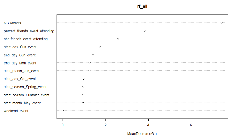
Understanding Variable Importance
We can study the Gini importances of the variables in our models.
varImpPlot(rf, type=2)
varImpPlot(rf_all, type=2)
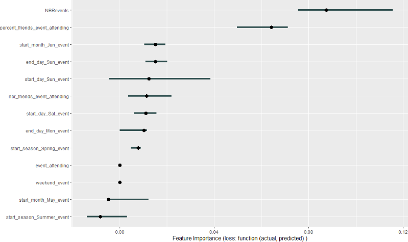
Using the IML Package for Variable Importance
The iml package can also be used for understanding variable importance.
We can use the FeatureImp function to do so.
p_load(iml)
iml_mod <- Predictor$new(
  model = rf_all,
  data = event_train,
  y = as.factor(event_train$event_attending),
  type = 'prob',
  class = 2
)

iml_imp <- FeatureImp$new(
  iml_mod,
  loss = function(actual, predicted) 1 - Metrics::auc(actual, predicted),
  compare = "difference"
)
plot(iml_imp)
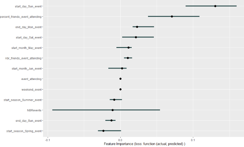
Or maybe have a look at the test set as well…
iml_test <- Predictor$new(
  model = rf_all,
  data = event_test,
  y = as.factor(event_test$event_attending),
  type = 'prob',
  class = 2
)

imp_test <- FeatureImp$new(
  iml_test,
  loss = function(actual, predicted) 1 - Metrics::auc(actual, predicted),
  compare = "difference"
)
plot(imp_test)
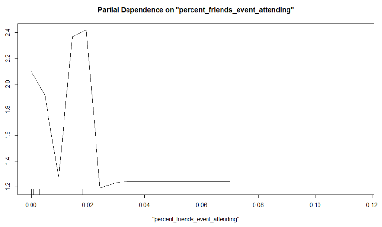
Partial Dependence Plots
Make a partial plot. Note that a partial plot does not work with a tibble, so that you need to transform the data to a dataframe.
partialPlot(
  x = rf_all,
  pred.data = data.frame(event_train),
  x.var = "percent_friends_event_attending",
  which.class = "1"
)
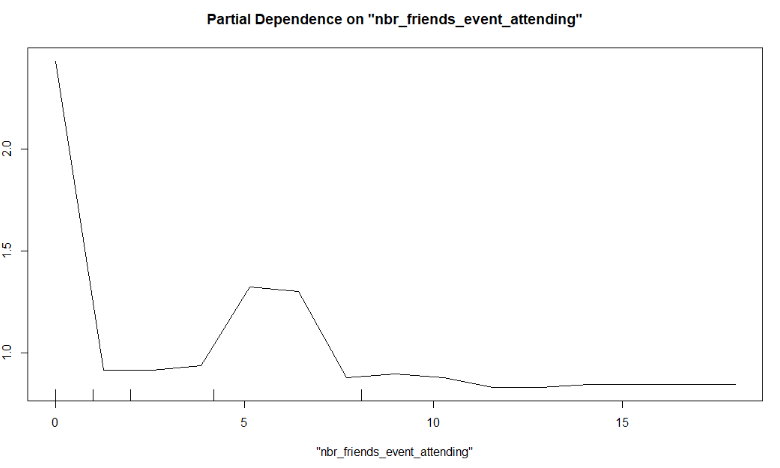
partialPlot(
  x = rf_all,
  pred.data = data.frame(event_train),
  x.var = "nbr_friends_event_attending",
  which.class = "1"
)
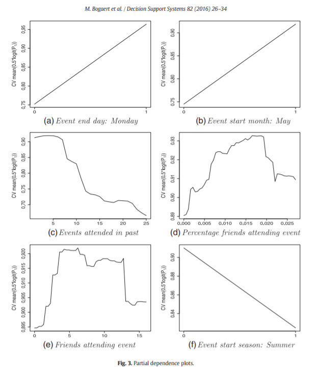
Multiple choice
Look at the partial dependency plots down below. Type the correct answer into the Dodona environment.
- When more friends are attending the event, a negative and afterwards a positive effect is observed.
- People are more likely to attend a soccer game in the summer.
- Soccer games that end on a Monday are not that popular.
- The propensity of attending an event will decline when you attend too many events.
To download the EventAttendance pdf click: here2