In this exercise you will create some simulated data and will fit simple linear regression models to it. Make sure to use set.seed(1) prior to starting to ensure consistent results.

Questions

Some of the exercises are not tested by Dodona (for example the plots), but it is still useful to try them.

1. Using the rnorm() function, create a vector x, containing 100 observations drawn from a \(N(0,1)\) distribution. This represents a feature, \(X\). Remember that the rnorm() takes the argument \(\mu\) and \(\sigma\), while the mathematical distribution is specified as \(N(\mu, \sigma^2)\)

2. Using the rnorm() function, create a vector eps, containing 100 observations drawn from a \(N(0, 0.25)\) distribution.

3. Using x and eps, generate a vector y according to the model \(Y = -1 + 0.5X + \varepsilon\) What is the length of the vector y? Store the value in y.length. What are the values of \(\beta_0\) and \(\beta_1\) in this linear model? Store them in beta0 and beta1.

4. Create a scatterplot displaying the relationship between x and y. Comment on what you observe.

5. Fit a least squares linear model to predict y using x. Store the model in lm.fit1. Comment on the model obtained. Store \(\hat{\beta}_0\) and \(\hat{\beta}_1\) in beta.hat0 and beta.hat1, respectively. How do \(\hat{\beta}_0\) and \(\hat{\beta}_1\) compare to \(\beta_0\) and \(\beta_1\)?

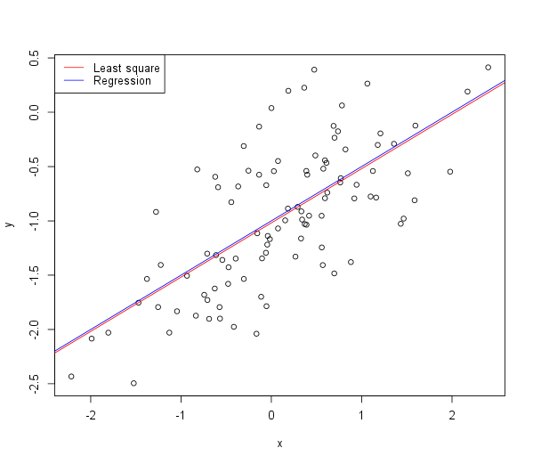
6. Display the least squares line on the scatterplot obtained in 5. Draw the population regression line on the plot, in a different color. Use the legend() function to create an appropriate legend.

   The plot should look like this:

   

7. Now fit a polynomial regression model that predicts \(y\) using \(x\) and \(x^2\). Store the model in lm.fit2.

8. MC1: Is there evidence that the quadratic term improves the model fit?
   1. Yes, the \(R^2\) is slightly higher and \(RSE\) slightly lower than the linear model.
   2. No, the coefficient for \(x^2\) is not significant as its p-value is higher than 0.05.
9. Repeat 1-6 after modifying the data generation process in such a way that there is less noise in the data \(eps2 ~ N(0, 0.125)\). The initial model should remain the same. MC2: Which of these statements is true (only one answer)?
   1. We have a much higher \(R^2\) and much lower $RSE$. Moreover, the two lines overlap each other as we have very little noise.
   2. We have a much lower \(R^2\) and much higher $RSE$. Moreover, the two lines are wider apart but are still really close to each other as we have a fairly large data set.
10. Repeat 1-6 after modifying the data generation process in such a way that there is more noise in the data \(eps3 ~ N(0, 0.5)\). The initial model should remain the same. MC3: Which of these statements is true (only one answer)?
    1. We have a much higher \(R^2\) and much lower \(RSE\). Moreover, the two lines overlap each other as we have very little noise.
    2. We have a much lower \(R^2\) and much higher \(RSE\). Moreover, the two lines are wider apart but are still really close to each other as we have a fairly large data set.
11. What are the confidence intervals for \(\beta_0\) and \(\beta_1\) based on the original data set, the noisier data set, and the less noisy data set? MC4: Which of these statements are false (only one answer)?
    1. All intervals seem to be centered on approximately 0.5
    2. As the noise increases, the confidence intervals widen.
    3. With less noise, there is less predictability in the data set.