In R, points falling outside the whiskers of the boxplot are referred to as outliers. This definition of outlier was introduced by Tukey. The top whisker ends at the 75th percentile plus 1.5 * IQR. Similarly the bottom whisker ends at the 25th percentile minus 1.5 * IQR. If we define the first and third quartiles as \(Q_1\) and \(Q_3\), respectively, then an outlier is anything outside the range:
\[[[Q_1 - 1.5 \times (Q_3 - Q1), Q_3 + 1.5 \times (Q_3 - Q1)]]\]When the data is normally distributed, the standard units of these values are:
q3 <- qnorm(0.75)
q1 <- qnorm(0.25)
iqr <- q3 - q1
r <- c(q1 - 1.5*iqr, q3 + 1.5*iqr)
r
#> [1] -2.7  2.7
Using the pnorm function, we see that 99.3% of the data falls in this
interval.
Keep in mind that this is not such an extreme event: if we have 1000 data points that are normally distributed, we expect to see about 7 outside of this range. But these would not be outliers since we expect to see them under the typical variation.
If we want an outlier to be rarer, we can increase the 1.5 to a larger
number. Tukey also used 3 and called these far out outliers. With a
normal distribution, 100% of the data falls in this interval. This
translates into about 2 in a million chance of being outside the range.
In the geom_boxplot function, this can be controlled by the
outlier.size argument, which defaults to 1.5.
The 180 inches measurement is well beyond the range of the height data:
max_height <- quantile(outlier_example, 0.75) + 3*IQR(outlier_example)
max_height
#>  75%
#> 6.91
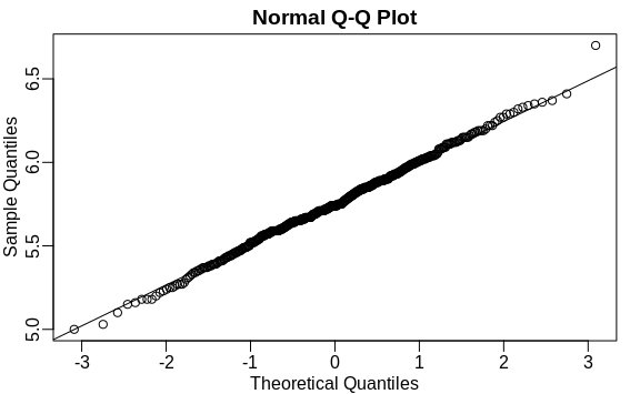
If we take this value out, we can see that the data is in fact normally distributed as expected:
x <- outlier_example[outlier_example < max_height]
qqnorm(x)
qqline(x)