Network Clustering in Social Network Analysis

Network clustering is a powerful tool in social network analysis that allows us to identify groups of nodes that are more densely connected to each other than to the rest of the network. In this exercise, we will explore network clustering using the igraph package in R, focusing on the Moreno and Facebook datasets.

Network Clustering Basics

Consider a network that has a variable which can be used as a clustering variable, such as gender. We will use the Moreno network as an example. The igraph package is loaded as it provides a wide range of options for community mining and clustering.

detach(package:statnet)
p_load(igraph)
data(Moreno)
iMoreno <- intergraph::asIgraph(Moreno)

To inspect the data, use the following statement.

table(V(iMoreno)$gender)

1   2
16  17

The modularity can then be calculated with clusters based on gender.

modularity(iMoreno,V(iMoreno)$gender)

0.4761342

Network Clustering with Facebook Data

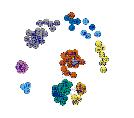
Another example is the Facebook data. The friends of a user are all given a label, depending on which group they belong to. Groups include friends, family, college friend, among others.

data(Facebook)
levels(factor(V(Facebook)$group))

"B" "C" "F" "G" "H" "M" "S" "W"

The “B” stands for book club, the “C” for college, the “F” for family, the “G” for graduate school, the “H” for high school, the “M” for music, the “S” for spiel (game) and the “W” for work. All these groups are in the data.

grp_num <- as.numeric(factor(V(Facebook)$group))
modularity(Facebook,grp_num)

0.6145798

The modularity is higher than that of the Moreno data set, meaning that a clustering based on groups leads to more dense clusters than clustering on gender.

To easily detect different communities, color can be added to the plot.

V(Facebook)$color <- grp_num
plot(Facebook)

Automatic Cluster Detection

In most cases, the clusters are not known. In order to automatically detect the number of clusters in a network, several algorithms have been proposed in literature. The most well-known algorithm is the Girvan-Newman algorithm which tries to maximizes the modularity to determine the optimal number of clusters.
Calculate the clusters based on edge betweenness (Girvan-Newman).

cw <- cluster_edge_betweenness(iMoreno)

Show the membership of clusters.

membership(cw)

1 1 1 1 2 2 1 1 2 3 2 3 3 3 3 1 2 4 4 4 5 5 5 4 4 4 4 4 4 4 5 6 6

Next, calculate modularity. Note that no clustering variable is required because a communities object is used and this object already determined the clusters.

modularity(cw)

0.6216919

To plot a communities object, first supply the community and then the graph object.

plot(cw, iMoreno)

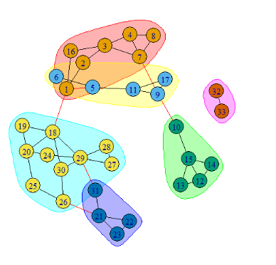
Several algorithms can be used and results can be compared. The algorithms can be compared both visually or with statistics. In se, clustering is a type of multiclass classification, and can similarly be evaluated. For more information about comparing clustering techniques, see the class of predictive analytics. For this class modularity is used as an evaluation metric, the higher, the better.

Assume that:

• The igraph library has been loaded.
• The facebook dataset from the UserNetR library has been loaded.
• The facebook data is an igraph object.