Using the histogram, density plots, and QQ-plots, we have become convinced that the male height data is well approximated with a normal distribution. In this case, we report back to ET a very succinct summary: male heights follow a normal distribution with an average of 69.3 inches and a SD of 3.6 inches. With this information, ET will have a good idea of what to expect when he meets our male students. However, to provide a complete picture we need to also provide a summary of the female heights.

We learned that boxplots are useful when we want to quickly compare two or more distributions. Here are the heights for men and women:

heights %>%
  ggplot(aes(x=sex, y=height, fill=sex)) +
  geom_boxplot()

The plot immediately reveals that males are, on average, taller than females. The standard deviations appear to be similar. But does the normal approximation also work for the female height data collected by the survey? We expect that they will follow a normal distribution, just like males. However, exploratory plots reveal that the approximation is not as useful:

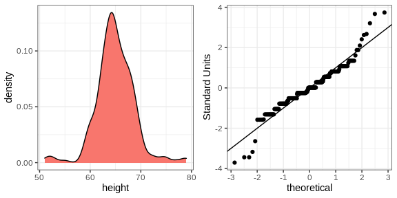
We see something we did not see for the males: the density plot has a second “bump”. Also, the QQ-plot shows that the highest points tend to be taller than expected by the normal distribution. Finally, we also see five points in the QQ-plot that suggest shorter than expected heights for a normal distribution. When reporting back to ET, we might need to provide a histogram rather than just the average and standard deviation for the female heights.

However, go back and read Tukey’s quote. We have noticed what we didn’t expect to see. If we look at other female height distributions, we do find that they are well approximated with a normal distribution. So why are our female students different? Is our class a requirement for the female basketball team? Are small proportions of females claiming to be taller than they are? Another, perhaps more likely, explanation is that in the form students used to enter their heights, FEMALE was the default sex and some males entered their heights, but forgot to change the sex variable. In any case, data visualization has helped discover a potential flaw in our data.

Regarding the five smallest values, note that these values are:

heights %>% filter(sex == "Female") %>%
  top_n(5, desc(height)) %>%
  pull(height)
#> [1] 51 53 55 52 52

Because these are reported heights, a possibility is that the student meant to enter 5'1", 5'2", 5'3" or 5'5".