In the previous section, we decided to perform this test only after examining the data
and noting that Managers One and Two had the highest and lowest mean
performances. In a sense, this means that we have implicitly performed
\(\binom{5}{2} = 5(5-1)/2 = 10\) hypothesis tests, rather than just one, as discussed
in Section 13.3.2. Hence, we use the TukeyHSD() function to apply Tukey’s
method in order to adjust for multiple testing. This function takes as input
the output of an ANOVA regression model, which is essentially just a linear
regression in which all of the predictors are qualitative. In this case, the
response consists of the monthly excess returns achieved by each manager,
and the predictor indicates the manager to which each return corresponds.
> returns <- as.vector(as.matrix(fund.mini))
> manager <- rep(c("1", "2", "3", "4", "5"), rep(50, 5))
> a1 <- aov(returns ~ manager)
> TukeyHSD(x = a1)
  Tukey multiple comparisons of means
    95% family-wise confidence level

Fit: aov(formula = returns ~ manager)

$manager
    diff        lwr       upr     p adj
2-1 -3.1 -6.9865435 0.7865435 0.1861585
3-1 -0.2 -4.0865435 3.6865435 0.9999095
4-1 -2.5 -6.3865435 1.3865435 0.3948292
5-1 -2.7 -6.5865435 1.1865435 0.3151702
3-2  2.9 -0.9865435 6.7865435 0.2452611
4-2  0.6 -3.2865435 4.4865435 0.9932010
5-2  0.4 -3.4865435 4.2865435 0.9985924
4-3 -2.3 -6.1865435 1.5865435 0.4819994
5-3 -2.5 -6.3865435 1.3865435 0.3948292
5-4 -0.2 -4.0865435 3.6865435 0.9999095
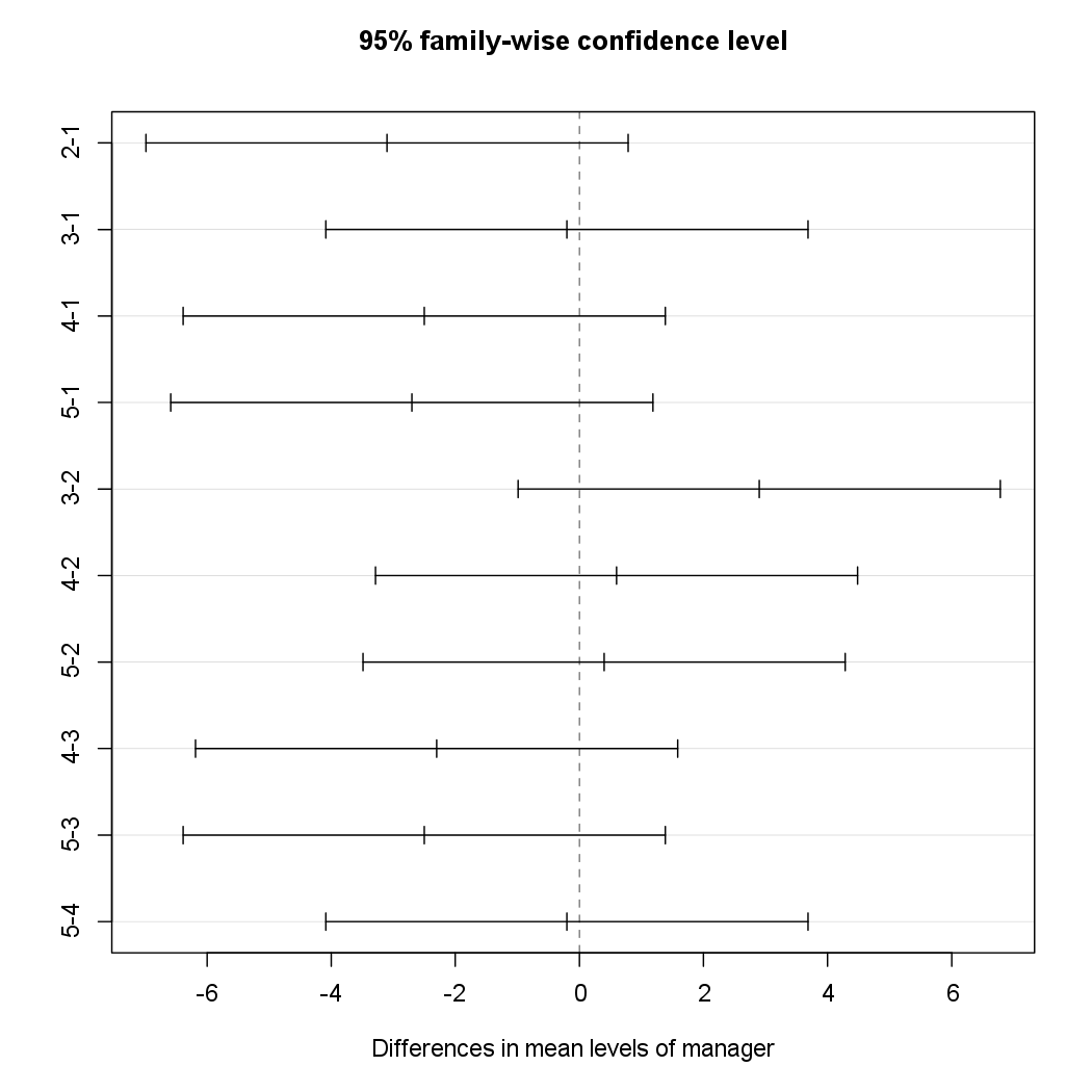
The TukeyHSD() function provides confidence intervals for the difference
between each pair of managers (lwr and upr), as well as a p-value. All of
these quantities have been adjusted for multiple testing. We can plot the confidence intervals
for the pairwise comparisons using the plot() function.
plot(TukeyHSD(x = a1))

Questions
- MC1: When adjusting for multiple testing, does the conclusion we made about the difference between manager 1 and 2 in the previous section change in any way?
1) there is still clear evidence of a difference between the managers’ performances.
2) there is no longer clear evidence of a difference between the managers’ performances.