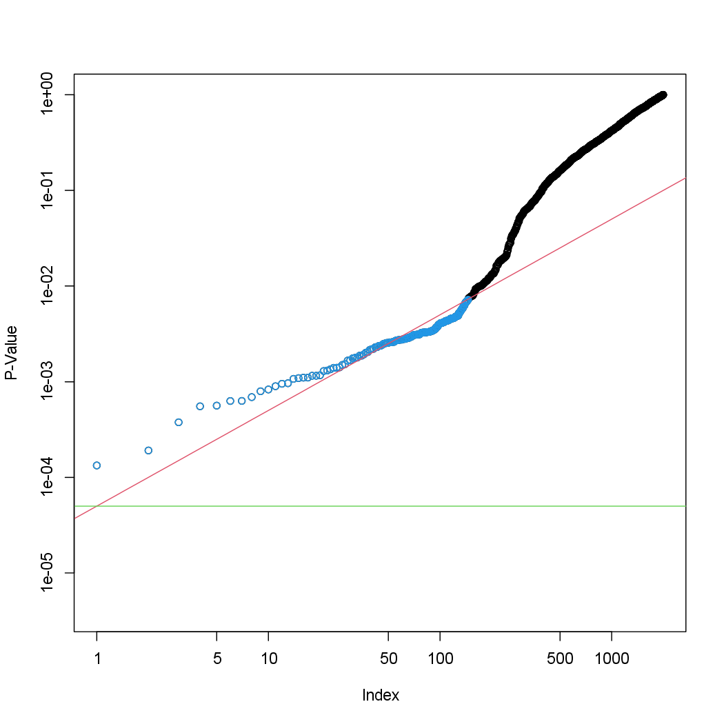
In the last section, we found that 146 of the 2,000 fund managers have a q-value below \(0.1\); therefore, we are able to conclude that 146 of the fund managers beat the market at an FDR of 10%. Only about 15 (10% of 146) of these fund managers are likely to be false discoveries. By contrast, if we had instead used Bonferroni’s method to control the FWER at level \(\alpha = 0.1\), then we would have failed to reject any null hypotheses!

> sum(fund.pvalues <= (0.1 / 2000))
[1] 0

Figure 13.6 displays the ordered p-values, \(p_{(1)} \leq p_{(2)} \leq \cdots \leq p_{(2000)}\), for the Fund dataset, as well as the threshold for rejection by the Benjamini- Hochberg procedure. Recall that the Benjamini-Hochberg procedure searches for the largest p-value such that \(p_{(j)} \le q_j/m\), and rejects all hypotheses for which the p-value is less than or equal to \(p_{(j)}\). In the code below, we implement the Benjamini-Hochberg procedure ourselves, in order to illustrate how it works. We first order the p-values. We then identify all p-values that satisfy \(p_{(j)} < q_j/m\) (wh.ps). Finally, wh indexes all p-values that are less than or equal to the largest p-value in wh.ps. Therefore, wh indexes the p-values rejected by the Benjamini-Hochberg procedure.

ps <- sort(fund.pvalues)
m <- length(fund.pvalues)
q <- 0.1
wh.ps <- which(ps < q * (1:m) / m)
if (length(wh.ps) > 0) {
  wh <- 1:max(wh.ps)
} else {
  wh <- numeric(0)
}

We now reproduce the middle panel of Figure 13.6.

plot(ps, log = "xy", ylim = c(4e-6, 1), ylab = "P-Value", xlab = "Index", main = "")
points(wh, ps[wh], col = 4)
abline(a = 0, b = (q / m), col = 2, untf = TRUE)
abline(h = 0.1 / 2000, col = 3)