The heights we have been looking at are not the original heights reported by students. The original reported heights are also included in the dslabs package and can be loaded like this:
library(dslabs)
data("reported_heights")
Height is a character vector so we create a new column with the numeric version:
reported_heights <- reported_heights %>%
  mutate(original_heights = height, height = as.numeric(height))
#> Warning: Problem with `mutate()` input `height`.
#> x NAs introduced by coercion
#> ℹ Input `height` is `as.numeric(height)`.
#> Warning in mask$eval_all_mutate(dots[[i]]): NAs introduced by coercion
Note that we get a warning about NAs. This is because some of the self reported heights were not numbers. We can see why we get these:
reported_heights %>% filter(is.na(height)) %>%  head()
#>            time_stamp    sex height original_heights
#> 1 2014-09-02 15:16:28   Male     NA            5' 4"
#> 2 2014-09-02 15:16:37 Female     NA            165cm
#> 3 2014-09-02 15:16:52   Male     NA              5'7
#> 4 2014-09-02 15:16:56   Male     NA            >9000
#> 5 2014-09-02 15:16:56   Male     NA             5'7"
#> 6 2014-09-02 15:17:09 Female     NA             5'3"
Some students self-reported their heights using feet and inches rather than just inches. Others used centimeters and others were just trolling. For now we will remove these entries:
reported_heights <- filter(reported_heights, !is.na(height))
If we compute the average and standard deviation, we notice that we obtain strange results. The average and standard deviation are different from the median and MAD:
reported_heights %>%
  group_by(sex) %>%
  summarize(average = mean(height), sd = sd(height),
            median = median(height), MAD = mad(height))
#> `summarise()` ungrouping output (override with `.groups` argument)
#> # A tibble: 2 x 5
#>   sex    average    sd median   MAD
#>   <chr>    <dbl> <dbl>  <dbl> <dbl>
#> 1 Female    63.4  27.9   64.2  4.05
#> 2 Male     103.  530.    70    4.45
This suggests that we have outliers, which is confirmed by creating a boxplot:
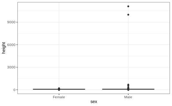
We can see some rather extreme values. To see what these values are, we
can quickly look at the largest values using the arrange function:
reported_heights %>% arrange(desc(height)) %>% top_n(10, height)
#>             time_stamp    sex height original_heights
#> 1  2014-09-03 23:55:37   Male  11111            11111
#> 2  2016-04-10 22:45:49   Male  10000            10000
#> 3  2015-08-10 03:10:01   Male    684              684
#> 4  2015-02-27 18:05:06   Male    612              612
#> 5  2014-09-02 15:16:41   Male    511              511
#> 6  2014-09-07 20:53:43   Male    300              300
#> 7  2014-11-28 12:18:40   Male    214              214
#> 8  2017-04-03 16:16:57   Male    210              210
#> 9  2015-11-24 10:39:45   Male    192              192
#> 10 2014-12-26 10:00:12   Male    190              190
#> 11 2016-11-06 10:21:02 Female    190              190
The first seven entries look like strange errors. However, the next few look like they were entered as centimeters instead of inches. Since 184 cm is equivalent to six feet tall, we suspect that 184 was actually meant to be 72 inches.
We can review all the nonsensical answers by looking at the data considered to be far out by Tukey:
whisker <- 3*IQR(reported_heights$height)
max_height <- quantile(reported_heights$height, .75) + whisker
min_height <- quantile(reported_heights$height, .25) - whisker
reported_heights %>%
  filter(!between(height, min_height, max_height)) %>%
  select(original_heights) %>%
  head(n=10) %>% pull(original_heights)
#>  [1] "6"     "5.3"   "511"   "6"     "2"     "5.25"  "5.5"   "11111"
#>  [9] "6"     "6.5"
Examining these heights carefully, we see two common mistakes: entries
in centimeters, which turn out to be too large, and entries of the form
x.y with x and y representing feet and inches, respectively, which
turn out to be too small. Some of the even smaller values, such as 1.6,
could be entries in meters.
In the Data Wrangling part of this book we will learn techniques for correcting these values and converting them into inches. Here we were able to detect this problem using careful data exploration to uncover issues with the data: the first step in the great majority of data science projects.