The visualizations above effectively illustrate that data no longer supports the western versus developing world view. Once we see these plots, new questions emerge. For example, which countries are improving more and which ones less? Was the improvement constant during the last 50 years or was it more accelerated during certain periods? For a closer look that may help answer these questions, we introduce time series plots.

Time series plots have time in the x-axis and an outcome or measurement of interest on the y-axis. For example, here is a trend plot of United States fertility rates:

gapminder %>% 
  filter(country == "United States") %>% 
  ggplot(aes(year, fertility)) +
  geom_point()

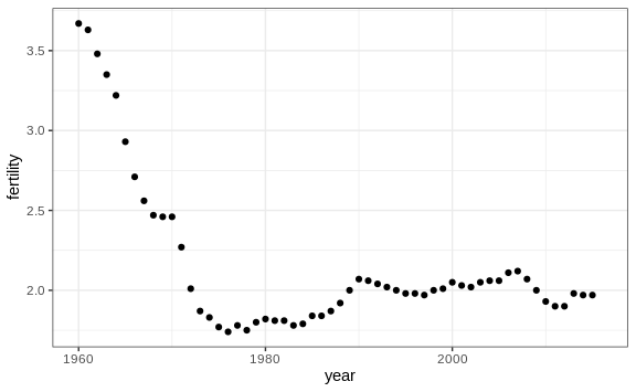
We see that the trend is not linear at all. Instead there is sharp drop during the 1960s and 1970s to below 2. Then the trend comes back to 2 and stabilizes during the 1990s.

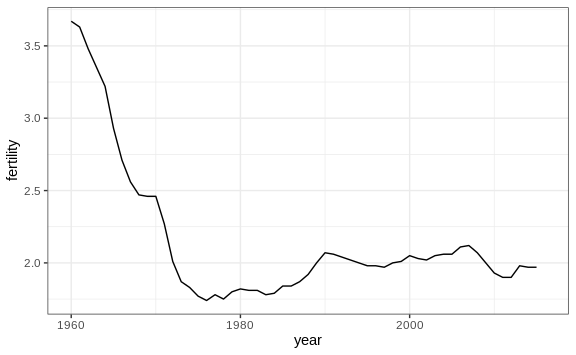
When the points are regularly and densely spaced, as they are here, we create curves by joining the points with lines, to convey that these data are from a single series, here a country. To do this, we use the geom_line function instead of geom_point.

gapminder %>% 
  filter(country == "United States") %>% 
  ggplot(aes(year, fertility)) +
  geom_line()

This is particularly helpful when we look at two countries. If we subset the data to include two countries, one from Europe and one from Asia, then adapt the code above:

countries <- c("South Korea","Germany")

gapminder %>% filter(country %in% countries) %>% 
  ggplot(aes(year,fertility)) +
  geom_line()

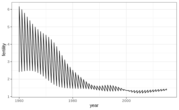
Unfortunately, this is not the plot that we want. Rather than a line for each country, the points for both countries are joined. This is actually expected since we have not told ggplot anything about wanting two separate lines. To let ggplot know that there are two curves that need to be made separately, we assign each point to a group, one for each country:

countries <- c("South Korea","Germany")

gapminder %>% filter(country %in% countries & !is.na(fertility)) %>% 
  ggplot(aes(year, fertility, group = country)) +
  geom_line()

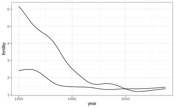
But which line goes with which country? We can assign colors to make this distinction. A useful side-effect of using the color argument to assign different colors to the different countries is that the data is automatically grouped:

countries <- c("South Korea","Germany")

gapminder %>% filter(country %in% countries & !is.na(fertility)) %>% 
  ggplot(aes(year,fertility, col = country)) +
  geom_line()

The plot clearly shows how South Korea’s fertility rate dropped drastically during the 1960s and 1970s, and by 1990 had a similar rate to that of Germany.

Labels instead of legends

For trend plots we recommend labeling the lines rather than using legends since the viewer can quickly see which line is which country. This suggestion actually applies to most plots: labeling is usually preferred over legends.

We demonstrate how we can do this using the life expectancy data. We define a data table with the label locations and then use a second mapping just for these labels:

labels <- data.frame(country = countries, x = c(1975,1965), y = c(60,72))

gapminder %>% 
  filter(country %in% countries) %>% 
  ggplot(aes(year, life_expectancy, col = country)) +
  geom_line() +
  geom_text(data = labels, aes(x, y, label = country), size = 5) +
  theme(legend.position = "none")

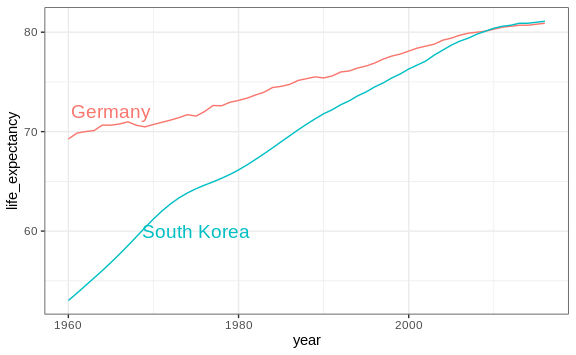
The plot clearly shows how an improvement in life expectancy followed the drops in fertility rates. In 1960, Germans lived 15 years longer than South Koreans, although by 2010 the gap is completely closed. It exemplifies the improvement that many non-western countries have achieved in the last 40 years.