Vaccines have helped save millions of lives. In the 19th century, before herd immunization was achieved through vaccination programs, deaths from infectious diseases, such as smallpox and polio, were common. However, today vaccination programs have become somewhat controversial despite all the scientific evidence for their importance.
The controversy started with a paper published in 1988 and led by Andrew Wakefield claiming there was a link between the administration of the measles, mumps, and rubella (MMR) vaccine and the appearance of autism and bowel disease. Despite much scientific evidence contradicting this finding, sensationalist media reports and fear-mongering from conspiracy theorists led parts of the public into believing that vaccines were harmful. As a result, many parents ceased to vaccinate their children. This dangerous practice can be potentially disastrous given that the Centers for Disease Control (CDC) estimates that vaccinations will prevent more than 21 million hospitalizations and 732,000 deaths among children born in the last 20 years (see Benefits from Immunization during the Vaccines for Children Program Era — United States, 1994-2013, MMWR). The 1988 paper has since been retracted and Andrew Wakefield was eventually “struck off the UK medical register, with a statement identifying deliberate falsification in the research published in The Lancet, and was thereby barred from practicing medicine in the UK.” (source: Wikipedia). Yet misconceptions persist, in part due to self-proclaimed activists who continue to disseminate misinformation about vaccines.
Effective communication of data is a strong antidote to misinformation and fear-mongering. Earlier we used an example provided by a Wall Street Journal article showing data related to the impact of vaccines on battling infectious diseases. Here we reconstruct that example.
The data used for these plots were collected, organized, and distributed by the Tycho Project. They include weekly reported counts for seven diseases from 1928 to 2011, from all fifty states. We include the yearly totals in the dslabs package:
library(tidyverse)
library(RColorBrewer)
library(dslabs)
data(us_contagious_diseases)
names(us_contagious_diseases)
#> [1] "disease"         "state"           "year"
#> [4] "weeks_reporting" "count"           "population"
We create a temporary object dat that stores only the measles data,
includes a per 100,000 rate, orders states by average value of disease
and removes Alaska and Hawaii since they only became states in the late
1950s. Note that there is a weeks_reporting column that tells us for
how many weeks of the year data was reported. We have to adjust for that
value when computing the rate.
the_disease <- "Measles"
dat <- us_contagious_diseases %>%
  filter(!state%in%c("Hawaii","Alaska") & disease == the_disease) %>%
  mutate(rate = count / population * 10000 * 52 / weeks_reporting) %>%
  mutate(state = reorder(state, rate))
We can now easily plot disease rates per year. Here are the measles data from California:
dat %>% filter(state == "California" & !is.na(rate)) %>%
  ggplot(aes(year, rate)) +
  geom_line() +
  ylab("Cases per 10,000")  +
  geom_vline(xintercept=1963, col = "blue")
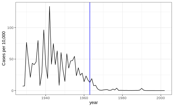
We add a vertical line at 1963 since this is when the vaccine was introduced [Control, Centers for Disease; Prevention (2014). CDC health information for international travel 2014 (the yellow book). p. 250. ISBN 9780199948505].
Now can we show data for all states in one plot? We have three variables to show: year, state, and rate. In the WSJ figure, they use the x-axis for year, the y-axis for state, and color hue to represent rates. However, the color scale they use, which goes from yellow to blue to green to orange to red, can be improved.
In our example, we want to use a sequential palette since there is no meaningful center, just low and high rates.
We use the geometry geom_tile to tile the region with colors
representing disease rates. We use a square root transformation to avoid
having the really high counts dominate the plot. Notice that missing
values are shown in grey. Note that once a disease was pretty much
eradicated, some states stopped reporting cases all together. This is
why we see so much grey after 1980.
dat %>% ggplot(aes(year, state, fill = rate)) +
  geom_tile(color = "grey50") +
  scale_x_continuous(expand=c(0,0)) +
  scale_fill_gradientn(colors = brewer.pal(9, "Reds"), trans = "sqrt") +
  geom_vline(xintercept=1963, col = "blue") +
  theme_minimal() +
  theme(panel.grid = element_blank(),
        legend.position="bottom",
        text = element_text(size = 8)) +
  ggtitle(the_disease) +
  ylab("") + xlab("")

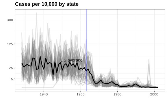
This plot makes a very striking argument for the contribution of vaccines. However, one limitation of this plot is that it uses color to represent quantity, which we earlier explained makes it harder to know exactly how high values are going. Position and lengths are better cues. If we are willing to lose state information, we can make a version of the plot that shows the values with position. We can also show the average for the US, which we compute like this:
avg <- us_contagious_diseases %>%
  filter(disease==the_disease) %>% group_by(year) %>%
  summarize(us_rate = sum(count, na.rm = TRUE) /
              sum(population, na.rm = TRUE) * 10000)
Now to make the plot we simply use the geom_line geometry:
dat %>%
  filter(!is.na(rate)) %>%
    ggplot() +
  geom_line(aes(year, rate, group = state),  color = "grey50",
            show.legend = FALSE, alpha = 0.2, size = 1) +
  geom_line(mapping = aes(year, us_rate),  data = avg, size = 1) +
  scale_y_continuous(trans = "sqrt", breaks = c(5, 25, 125, 300)) +
  ggtitle("Cases per 10,000 by state") +
  xlab("") + ylab("") +
  geom_text(data = data.frame(x = 1955, y = 50),
            mapping = aes(x, y, label="US average"),
            color="black") +
  geom_vline(xintercept=1963, col = "blue")
In theory, we could use color to represent the categorical value state, but it is hard to pick 50 distinct colors.