Here, we implement the re-sampling approach to hypothesis testing using
the Khan dataset, which we investigated in Section 13.5. First, we merge
the training and testing data, which results in observations on 83 patients
for 2,308 genes.
> attach(Khan)
> x <- rbind(xtrain, xtest)
> y <- c(as.numeric(ytrain), as.numeric(ytest))
> dim(x)
[1]   83 2308
> table(y)
y
 1  2  3  4
11 29 18 25
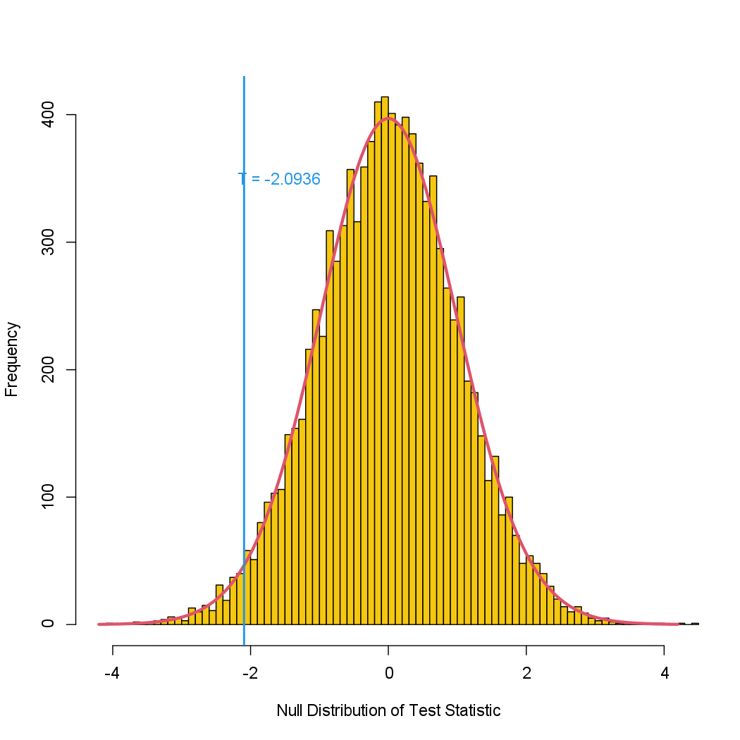
There are four classes of cancer. For each gene, we compare the mean expression in the second class (rhabdomyosarcoma) to the mean expression in the fourth class (Burkitt’s lymphoma). Performing a standard two-sample t-test on the 11th gene produces a test-statistic of \(−2.09\) and an associated p-value of \(0.0412\), suggesting modest evidence of a difference in mean expression levels between the two cancer types.
> x <- as.matrix(x)
> x1 <- x[which(y == 2),]
> x2 <- x[which(y == 4),]
> n1 <- nrow(x1)
> n2 <- nrow(x2)
> t.out <- t.test(x1[, 11], x2[, 11], var.equal = TRUE)
> TT <- t.out$statistic
> TT
        t
-2.093633
> t.out$p.value
[1] 0.04118644
However, this p-value relies on the assumption that under the null hypothesis of no difference between the two groups, the test statistic follows a t-distribution with \(29 + 25 - 2 = 52\) degrees of freedom. Instead of using this theoretical null distribution, we can randomly split the \(54\) patients into two groups of \(29\) and \(25\), and compute a new test statistic. Under the null hypothesis of no difference between the groups, this new test statistic should have the same distribution as our original one. Repeating this process 10,000 times allows us to approximate the null distribution of the test statistic. We compute the fraction of the time that our observed test statistic exceeds the test statistics obtained via re-sampling.
> set.seed(1)
> B <- 10000
> Tbs <- rep(NA, B)
> for (b in 1:B) {
+   dat <- sample(c(x1[, 11], x2[, 11]))
+   Tbs[b] <- t.test(dat[1:n1], dat[(n1 + 1):(n1 + n2)], var.equal = TRUE)$statistic
+ }
> mean((abs(Tbs) >= abs(TT)))
[1] 0.0416
This fraction, \(0.0416\), is our re-sampling-based p-value. It is almost identical to the p-value of \(0.0412\) obtained using the theoretical null distribution.
We can plot a histogram of the re-sampling-based test statistics.
hist(Tbs, breaks = 100, xlim = c(-4.2, 4.2), main = "",
     xlab = "Null Distribution of Test Statistic", col = 7)
lines(seq(-4.2, 4.2, len = 1000), dt(seq(-4.2, 4.2, len = 1000), df = (n1 + n2 - 2)) * 1000, col = 2, lwd = 3)
abline(v = TT, col = 4, lwd = 2)
text(TT + 0.5, 350, paste("T = ", round(TT, 4), sep = ""), col = 4)
Questions
- Perform the same analysis on gene 20.
- Store the two-sample t-test test-statistic in
TTand p-value intt.pvalue. - Approximate the null distribution of the test statistic by repeating the process 10000 times.
Store the re-sampling p-value in
rs.pvalue. Use a seed value of 1.
Assume that:
- The
ISLR2library has been loaded - The
Khandataset has been loaded and attached