Drop hier links of afbeeldingen om ze aan de editor toe te voegen.
Topics and Terms
After creating the LDA model, we can inspect the topics and terms.
We’ll use the tidy function to neatly output the beta matrix.
(topic_term <- tidy(topicmodel, matrix = 'beta'))
# A tibble: 9,184 x 3
   topic    term            beta
   <int>    <chr>           <dbl>
 1     1    pay        1.52e- 50
 2     2    pay        4.70e- 57
 3     3    pay        1.22e-  2
 4     4    pay        5.55e-177
 5     1    black      3.25e- 28
 6     2    black      5.65e-  4
 7     3    black      1.32e-156
 8     4    black      2.61e-  3
 9     1    history    1.12e-  3
10     2    history    1.47e-  3
# ... with 9,174 more rows
Each row represents a topic per term. For example, pay has a probability of 1.52e-50 to belong to topic 1.
Identifying Top Terms per Topic
We can also identify the top ten terms per topic.
top_terms <- topic_term %>%
  group_by(topic) %>%
  top_n(10, beta) %>%
  ungroup() %>%
  arrange(topic, desc(beta))
top_terms
# A tibble: 40 x 3
   topic    term              beta
   <int>    <chr>             <dbl>
 1     1    republicans     0.0229
 2     1    roe             0.0206
 3     1    house           0.0152
 4     1    social          0.0148
 5     1    security        0.0140
 6     1    democrats       0.0133
 7     1    wade            0.0129
 8     1    codify          0.0124
 9     1    law             0.0121
10     1    protect         0.0119
# ... with 30 more rows
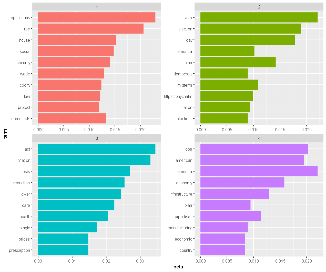
Visualizing Top Terms
These top ten terms per topic can be visualized using a bar plot.
top_terms %>%
  mutate(term = reorder(term, beta)) %>%
  ggplot(aes(term, beta, fill = factor(topic))) +
  geom_col(show.legend = FALSE) +
  facet_wrap(~ topic, scales = "free") +
  coord_flip()
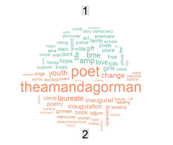
Creating a Word Cloud
We can also create a word cloud for a more intuitive understanding of the top terms.
topic_term %>%
  group_by(topic) %>%
  top_n(50, beta) %>%
  pivot_wider(term, topic, values_from = "beta", names_prefix = 'topic', values_fill = 0) %>%
  column_to_rownames("term") %>%
  comparison.cloud(colors = brewer.pal(3, "Set2"))

Exercise
Down below, a wordcloud for the two topics is presented.
Get the topic per term and their probabilities.
Store this in topic_per_term.
Then, get the top 5 terms per topic and their beta coefficient and store this in top.
To download the topicmodel click: here
Assume that:
- The
topicmodelfrom the previous exercise has been loaded. - All the packages to perform topic modeling have been loaded.