Next we consider the task of predicting whether an individual earns more than $250,000 per year. We proceed much as before, except that first we create the appropriate response vector, and then apply the glm() function using family="binomial" in order to fit a polynomial logistic regression model.

fit <- glm(I(wage > 250) ~ poly(age, 4), data = Wage, family = binomial)

Note that we again use the wrapper I() to create this binary response variable on the fly. The expression wage>250 evaluates to a logical variable containing TRUEs and FALSEs, which glm() coerces to binary by setting the TRUEs to 1 and the FALSEs to 0.

Once again, we make predictions using the predict() function.

preds <- predict(fit, newdata = list(age = age.grid), se = TRUE)

However, calculating the confidence intervals is slightly more involved than in the linear regression case. The default prediction type for a glm() model is type="link", which is what we use here. This means we get predictions for the logit: that is, we have fit a model of the form

\[\log \left( \frac{\Pr(Y = 1 \mid X)}{1 - \Pr(Y = 1 \mid X)} \right) = X \beta,\]

and the predictions given are of the form \(X \beta\). The standard errors given are also of this form. In order to obtain confidence intervals for \(\Pr(Y = 1 \mid X)\), we use the transformation

\[\Pr(Y = 1 \mid X) = \frac{\exp(X \beta)}{1 + \exp(X \beta)}.\]

pfit <- exp(preds$fit) / (1 + exp(preds$fit))
se.bands.logit <- cbind(preds$fit + 2 * preds$se.fit, preds$fit - 2 * preds$se.fit)
se.bands <- exp(se.bands.logit) / (1 + exp(se.bands.logit))

Finally, the plot below is made as follows:

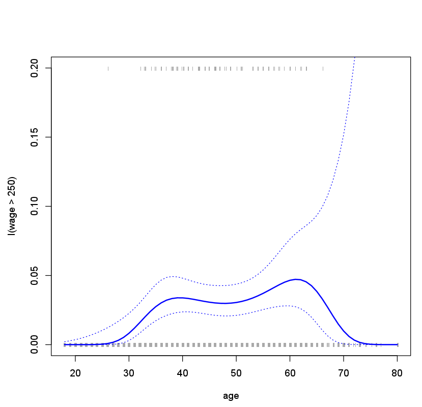
plot(age, I(wage > 250), xlim = agelims, type = "n", ylim = c(0, .2))
points(jitter(age), I((wage > 250) / 5), cex = .5, pch = "|", col = "darkgrey")
lines(age.grid, pfit, lwd = 2, col = "blue")
matlines(age.grid, se.bands, lwd = 1, col = "blue", lty = 3)

We have drawn the age values corresponding to the observations with wage values above 250 as gray marks on the top of the plot, and those with wage values below 250 are shown as gray marks on the bottom of the plot. We used the jitter() function to jitter the age values a bit so that observations with the same age value do not cover each other up. This is often called a rug plot.

Questions

• Create a polynomial logistic regression that predicts whether a neighbourhood has a median housing price larger than $30,000. Use the Boston dataset with medv as dependent variable and a degree-3 polynomial of dis as independent variable (weighted mean of distances to five Boston employment centres). Use the orthogonal polynomials and keep in mind that the median value medv is displayed in $1000s. Store the result in fit.
• Calculate the predictions of medv for a series of values of dis, ranging from 1 mile to 12 miles, in steps of 0.1 mile. Store the results in the variable preds.
• Transform the fitted probabilities and store the result in pfit.
• Calculate the confidence intervals with z-value 2.0. Store the results in variable se.bands. Remember to transform the confidence intervals.

Assume that:

• The MASS library has been loaded
• The Boston dataset has been loaded and attached