Variable Importance in Random Forest

In this exercise, we will delve into the concept of variable importance in the context of the random forest algorithm in R. The randomForest, AUC and iml packages are required for this exercise. We will use the data_sets.Rdata to illustrate the concept of variable importance.

Loading Required Packages and Data

if (!require("pacman")) install.packages("pacman"); require("pacman")
p_load(tidyverse, randomForest, iml)

Building the Random Forest Model

To be able to extract the variable importance, a random forest model needs to be constructed with importance = TRUE.

rFmodel <- randomForest(
  x = BasetableTRAIN,
  y = yTRAIN,
  ntree = 1000,
  importance = TRUE
)

Understanding Variable Importance

Variable importance is a key aspect of a random forest model. It allows us to understand which variables contribute the most to the model’s predictive power. We can extract the variable importance from our model using the importance function.

importance(rFmodel, type = 1)
importance(rFmodel, type = 2)

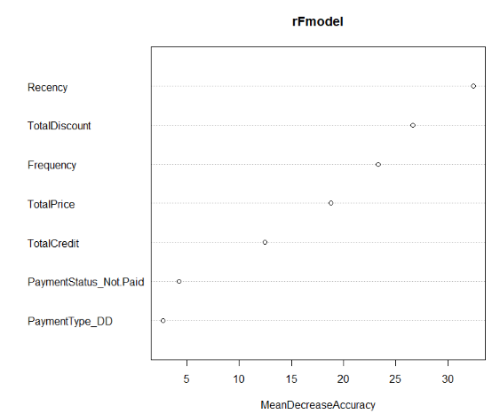
importance(rFmodel, type = 1)
                                  MeanDecreaseAccuracy
TotalDiscount                     26.623587
TotalPrice                        18.805011
TotalCredit                       12.464571
PaymentType_DD                    2.7294190
PaymentStatus_Not.Paid            4.2369690
Frequency                         23.301393
Recency                           32.408494

importance(rFmodel, type = 2)
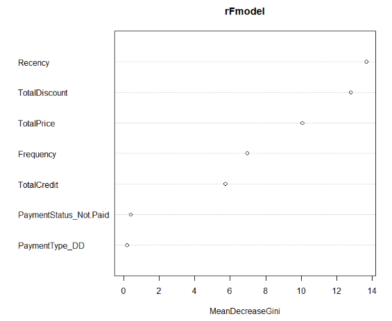
                                  MeanDecreaseGini
TotalDiscount                     12.8097503
TotalPrice                        10.0593459
TotalCredit                       5.72686520
PaymentType_DD                    0.17638050
PaymentStatus_Not.Paid            0.38232450
Frequency                         6.94735730
Recency                           13.6770525

A nice tabular view of the importances can be obtained by the following code block.

(impAcc <- importance(rFmodel, type = 1) %>%
  as_tibble(., rownames = 'Features') %>%
  arrange(desc(MeanDecreaseAccuracy)))
(impGini <- importance(rFmodel, type = 2) %>%
  as_tibble(., rownames = 'Features') %>%
  arrange(desc(MeanDecreaseGini)))

Features                    MeanDecreaseAccuracy
1 Recency                   32.4 
2 TotalDiscount             26.6 
3 Frequency                 23.3 
4 TotalPrice                18.8 
5 TotalCredit               12.5 
6 PaymentStatus_Not.Paid    4.24
7 PaymentType_DD            2.73

Features                    MeanDecreaseGini
1 Recency                   13.7  
2 TotalDiscount             12.8  
3 TotalPrice                10.1  
4 Frequency                 6.95 
5 TotalCredit               5.73 
6 PaymentStatus_Not.Paid    0.382
7 PaymentType_DD            0.176

Visualizing Variable Importance

Visualizing the variable importance can provide a more intuitive understanding. We can create a dot plot of the variable importance.

varImpPlot(rFmodel, type = 1)
varImpPlot(rFmodel, type = 2)

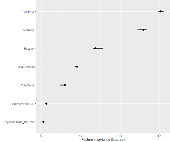
Using the iml Package

Also, the iml package can be used. This is a more general interpretable machine learning package. It allows you to calculate feature importance by several loss functions and for any model. The FeatureImp function has several loss functions based on the metrics package library(help = "Metrics").

First, create a predictor object. We specify class 2 since we want to get our second factor (i.e. 1).

mod <- Predictor$new(
  model = rFmodel,
  data = BasetableTRAIN,
  y = yTRAIN,
  type = 'prob', 
  class = 2
)

Next, create a new object with loss function. We create the loss function with classification error (or 1 - accuracy). Since the model always calculates the increase in error, calculating the increase in classification error is the same as calculating the decrease in accuracy.

(imp <- FeatureImp$new(mod, loss = 'ce'))

Interpretation method:  FeatureImp 
error function: ce

Analysed predictor: 
Prediction task: unknown 

Analysed data:
Sampling from data.frame with 707 rows and 7 columns.

Head of results:
    feature         importance.05  importance   importance.95   permutation.error
1   TotalPrice      1.594410       1.605590     1.622981        0.7312588
2   Frequency       1.488820       1.518634     1.536025        0.6916549
3   Recency         1.263975       1.273292     1.313043        0.5799151
4   TotalDiscount   1.168944       1.180124     1.185714        0.5374823
5   TotalCredit     1.093168       1.118012     1.122981        0.5091938
6   PaymentType_DD  1.022360       1.024845     1.024845        0.4667610

Confidence bands 5 % and 95 % are also reported. The importance column is the median permutation importance over 5 repetitions runs. By default, the ratio in model error is reported. The difference in model can be seen by adding compare = 'difference'.

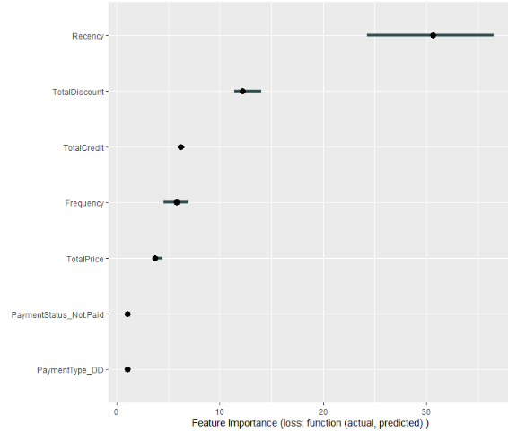
A plot can be made as well.

plot(imp)

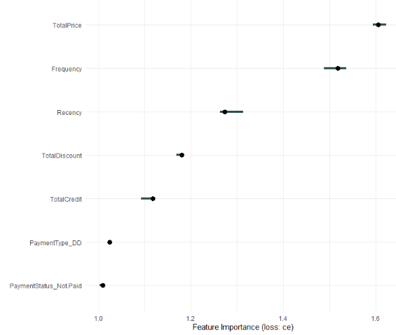
This is a ggplot object, so you can play around with it.

plot(imp) + theme_minimal()

For another measure like AUC, create your own loss function.

imp <- FeatureImp$new(mod, loss = function(actual, predicted) 1 - Metrics::auc(actual, predicted))
plot(imp)

To download the Covid-19 data click: here¹

Assume that:

• The randomForest library has been loaded.
• The Covid-19 data has been loaded.