One can also plot the cross-validation scores using the validationplot()
function. Using val.type="MSEP" will cause the cross-validation \(MSE\) to be
plotted.
validationplot(pcr.fit, val.type = "MSEP")
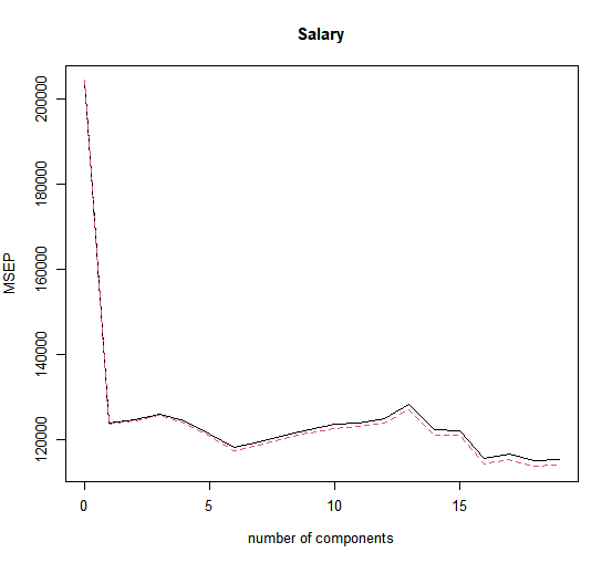
We see that the smallest cross-validation error occurs when \(M = 16\) components are used. This is barely fewer than \(M = 19\), which amounts to simply performing least squares, because when all of the components are used in PCR no dimension reduction occurs. However, from the plot we also see that the cross-validation error is roughly the same when only one component is included in the model. This suggests that a model that uses just a small number of components might suffice.
The summary() function also provides the percentage of variance explained
in the predictors and in the response using different numbers of components.
This concept is discussed in greater detail in Chapter 10. Briefly,
we can think of this as the amount of information about the predictors or
the response that is captured using \(M\) principal components. For example,
setting \(M = 1\) only captures 38.31% of all the variance, or information, in
the predictors. In contrast, using \(M = 6\) increases the value to 88.63%. If
we were to use all \(M = p = 19\) components, this would increase to 100%.
Questions
Here you see the summary() function applied to the pcr model you created in the previous exercise:
> summary(pcr.fit)
Data: 	X dimension: 506 13
	Y dimension: 506 1
Fit method: svdpc
Number of components considered: 13

VALIDATION: RMSEP
Cross-validated using 10 random segments.
       (Intercept)  1 comps  2 comps  3 comps  4 comps  5 comps
CV           9.206    7.303    6.969    5.619    5.588    5.204
adjCV        9.206    7.301    6.966    5.613    5.636    5.193
           6 comps  7 comps  8 comps  9 comps  10 comps  11 comps
CV           5.185    5.187    5.164    5.187     5.213     5.179
adjCV        5.175    5.178    5.155    5.178     5.201     5.166
          12 comps  13 comps
CV           5.023     4.944
adjCV        5.009     4.930

TRAINING: % variance explained
      1 comps  2 comps  3 comps  4 comps  5 comps
X       47.13    58.15    67.71    74.31    80.73
medv    37.42    45.59    63.59    64.78    69.70
      6 comps  7 comps  8 comps  9 comps  10 comps
X       85.79    89.91    92.95    95.08     96.78
medv    70.05    70.05    70.56    70.57     70.89
     11 comps  12 comps  13 comps
X       98.21     99.51    100.00
medv    71.30     73.21     74.06
MC1:
A) Using \(M = 4\) captures 64.78% of the variance in X
B) Using \(M = 11\) captures 98.21% of the variance in X
- 1) Both statements are true.
- 2) Both statements are false.
- 3) A is true and B is false.
- 4) A is false and B is true.