If we type,
par(mfrow = c(2, 2))
plot(lm.fit2)
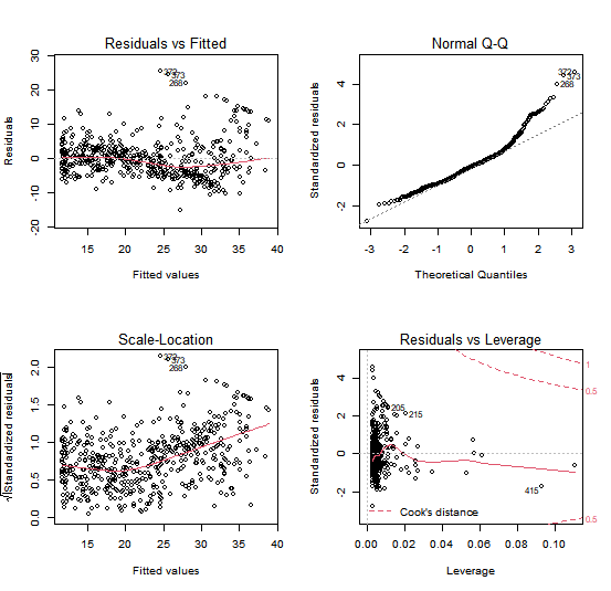
we see that when the lstat² term is included in the model, there is
little discernible pattern in the residuals.
In order to create a cubic fit, we can include a predictor of the form
I(X^3). However, this approach can start to get inconvenient for higher-order polynomials.
A better approach involves using the poly() function to create the polynomial within lm().
For example, the following command produces a fifth-order polynomial fit:
lm.fit5 <- lm(medv ~ poly(lstat, 5))
summary(lm.fit5)

Call:
lm(formula = medv ~ poly(lstat, 5))

Residuals:
     Min       1Q   Median       3Q      Max
-13.5433  -3.1039  -0.7052   2.0844  27.1153

Coefficients:
                 Estimate Std. Error t value Pr(>|t|)
(Intercept)       22.5328     0.2318  97.197  < 2e-16 ***
poly(lstat, 5)1 -152.4595     5.2148 -29.236  < 2e-16 ***
poly(lstat, 5)2   64.2272     5.2148  12.316  < 2e-16 ***
poly(lstat, 5)3  -27.0511     5.2148  -5.187 3.10e-07 ***
poly(lstat, 5)4   25.4517     5.2148   4.881 1.42e-06 ***
poly(lstat, 5)5  -19.2524     5.2148  -3.692 0.000247 ***
---
Signif. codes:  0 ‘***’ 0.001 ‘**’ 0.01 ‘*’ 0.05 ‘.’ 0.1 ‘ ’ 1
This suggests that including additional polynomial terms, up to fifth order, leads to an improvement in the model fit! However, further investigation of the data reveals that no polynomial terms beyond fifth order have significant p-values in a regression fit.
Try creating a model that predicts medv with a fourth-order polynomial of the crim variable using the poly() function:
Assume that:
- The
MASSlibrary has been loaded - The
Bostondataset has been loaded and attached